Define the observational unit (rows) and variables (columns) of rectangular data
Identify variable types given rectangular data
Explore rectangular data quickly in R (with code and with RStudio visually)
Read rectangular data with various delimiters into R using an appropriate readr or readxl function
Define relative versus absolute file paths
5.1 Rectangular Data
There are a lot of different ways that we can look at data in the world and store it on our computer. In this class, we will primarily focus on working with what we call rectangular data meaning that the data is two-dimentional with rows and columns. With rectangular data, each row represents one observation (or observational unit) and each column represents a variable.
There are also multiple ways that rectangular data can be stored in R! We will primarily work with data.frame() and tibble() ojects. It is important to know the type and format of the data you’re working with! It is much easier to create data visualizations or conduct statistical analyses if the data you use is in the right shape.
In a perfect world, all data would come in the right format for our needs, but this is often not the case. We will spend the next few weeks learning about how to use R to read in data and reformat our data so that it can be used in a specific analysis.
5.1.1 Data Frames in R
Data frames are a specific object type in R, data.frame(), and can be indexed the same as matrices. It may be useful to actually look at your data before beginning to work with it to see the format of the data. The following functions in R help us learn information about our data sets:
class(): outputs the object type
names(): outputs the variable (column) names
head(): outputs the first 6 rows of a dataframe
glimpse() or str(): output a transpose of dataframe or matrix; shows the data types
summary() outputs 6-number summaries or frequencies for all variables in the data set depending on the variables data type
data$variable: extracts a specific variable (column) from the data set
You may also choose to click on the data set name in your Environment window pane in R and the data set will pop up in a new tab in the script pane.
Let’s start with looking at a dataset that is included in a package in R.
The cereal dataset is included in the liver package. To open this dataset, we nead to load the package liver first, and then we can use the data() function to look at the cereal data.
# load liver packagelibrary(liver)# load cereal data which is included in the packagedata(cereal)# look at the first couple of rowshead(cereal)
What kinds of variables are available in the data? How many are there?
What questions do you have about the variables after just looking at the data?
Just looking at a data frame in R, we can’t tell how the variables are measures and what they all mean! We will always want to look at a data dictionary to understand what the columns really mean. Any good data provider should provide a data dictionary along with the data!
In this case, we can find the data dictionary in the help file for the data in R by running:
?cereal
Check In
According to the data dictionary, what does a row represent in the data?
What does the variable shelf measure and what are the possible values? Should this be treated as a categorical or a numeric variable?
What is the unit for the sodium variable? What about fiber?
5.2 Reading in Data
In order to use statistical software to do anything interesting, we need to be able to get data into the program so that we can work with it effectively.
5.2.1 File Paths
Before we can read in data, we need to tell R where to look for the data file!
A file path describes where a certain file or directory lives on your computer. Any time that you are working in R, there is a working directory, which is the baseline directory that R is then looking for other files from. You can find your current working directory with:
There are two different kinds of file paths that you can define to indicate the location of a file or directory:
absolute file path: full path from the root directory on your computer. Note this will only work on your computer!
relative file path: path based on the relationship with a current working directory in terms of a hierarchichy of directories
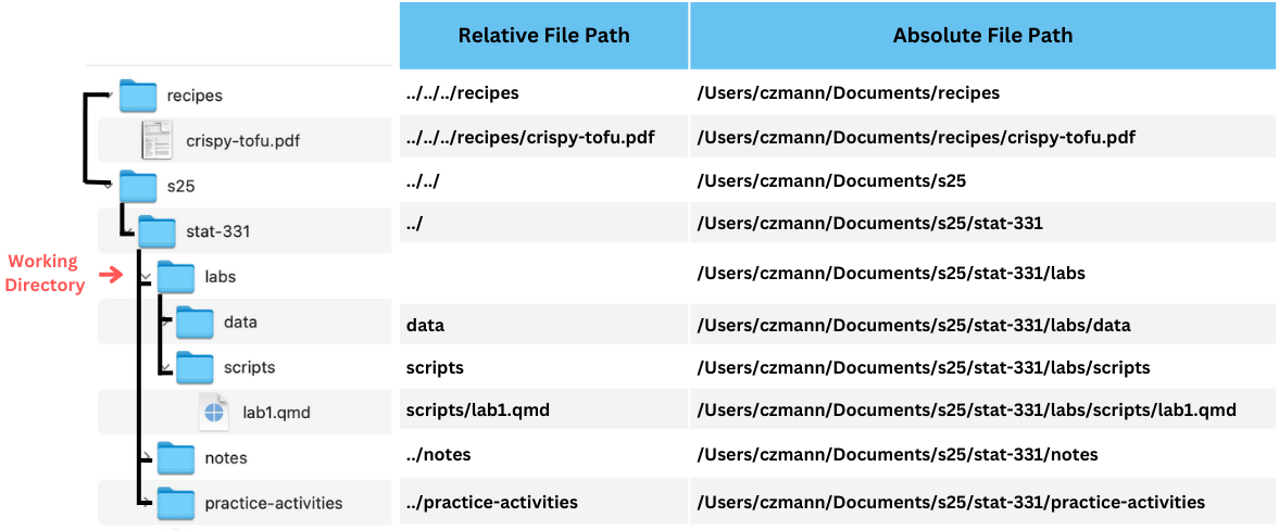
Let’s look at an example of relative versus absolute file paths. In the example below the “labs” directory is the working directory. The directories that “labs” are in are called it’s parent directories, which are referenced with "../" in the relative file paths.
Important
Since absolute file paths only work on your computer, we will always use relative file paths in this course.
5.2.2 Types of Data Files
We will also need to tell R what kind of data it an expect. In this class, are focusing on rectangular data, with rows indicating observations and columns that show variables. This type of data can be stored on the computer in multiple ways which indicate rows and columns in different ways:
as raw text, usually in a file that ends with .txt, .tsv, .csv, .dat, or sometimes, there will be no file extension at all.
.csv “Comma-separated”
.txt plain text
rows will always be separated in new lines
columns can be separated with different delimiters including tabs, spaces, commas, or other delimeters
in a spreadsheet. Spreadsheets, such as those created by MS Excel, Google Sheets use a special type of markup that is specific to the filetype and the program it’s designed to work with. Therefore, special functionality is required for working with them in R.
.xls
.xlsx
To work with data in R, it’s important to know how to read in text files (CSV, tab-delimited, etc.). It can be helpful to also know how to read in XLSX files.
Let’s practice recognizing different kinds of data files.
Check In
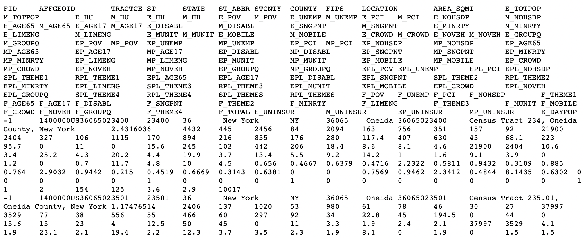
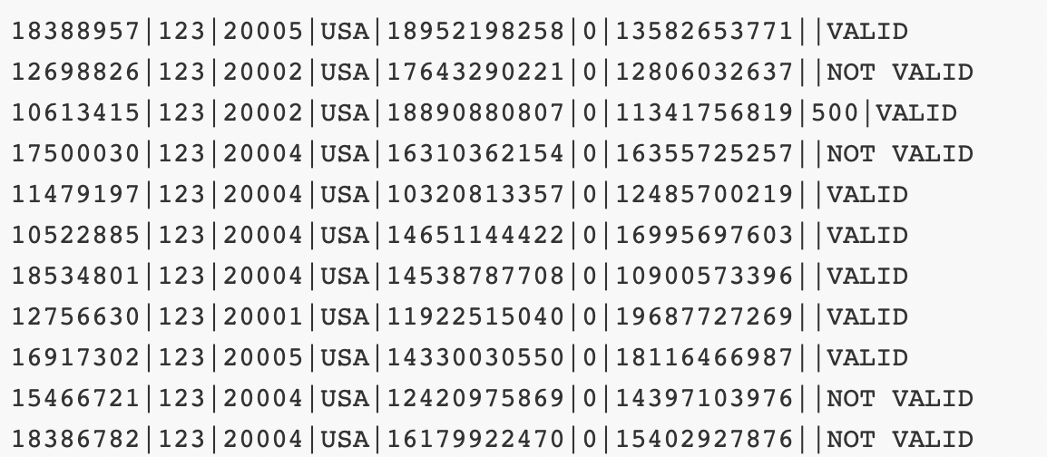
What kind of data file are each of the following? Note what kind of delimeter is used to separate columns.
Note: there are a lot of other ways to store data that we just won’t talk about in this class!
5.2.3 Reading in Data with readr and readxl
read_csv() is for reading in .csv files
read_txv() is for tab-separated data
read_table() is for any data with “columns” (white space separating)
read_delim() is for special “delimiters” separating data
read_xlsx() is specifically for dealing with Excel files
# load the readr package (or alternatively the tidyverse package)library(readr)# here we are using a URLsurveys <-read_csv(file ="https://raw.githubusercontent.com/earobinson95/stat331-calpoly/master/lab-assignments/Lab2-graphics/surveys.csv")# here is an example of a relative file path to an actual data file!surveys <-read_csv(file ="../data/surveys.csv")